Variational Inference
Posted on Aug 16, 2019
Variational Inference (VI) is a strategy to approximate difficult-to-compute probability densities (Blei et al., 2017). Being an alternative method to the Markov chain Monte Carlo sampling (MCMC), it is widely used in Bayesian models to compute the approximate posterior probability densities. Its applications encompass computer vision, computational neuro-science and large scale document analysis (Srivastava and Sutton, 2017; Kendall and Gal, 2017).
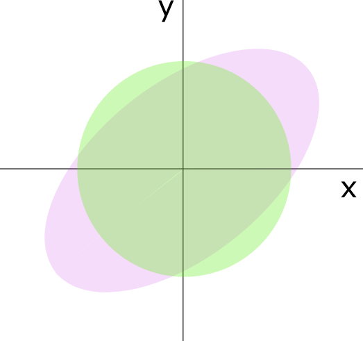
Consider the following problem of modeling the joint density of the latent variables \(\mathbf{z} = z_{1:m}\) and observations \(\mathbf{x} = x_{1:n}\), \begin{align} p(\mathbf{x}, \mathbf{z}) = \underbrace{p(\mathbf{x} | \mathbf{z})}_{\text{likelihood}} \, \underbrace{p(\mathbf{z})}_{\text{prior}} \end{align} The latent variables help explain the distribution of the observations. Models described by above equation draw samples from the prior distribution and relate them to the likelihood of the observations. Inference in such models involves the computation of the posterior, \(p(\mathbf{z} | \mathbf{x})\). We can write the conditional density as follows, \begin{align} p_{\theta}(\mathbf{z} | \mathbf{x}) &= \frac{p_{\theta}(\mathbf{z}, \mathbf{x})}{p_{\theta}(\mathbf{x})} \end{align} where the marginal distribution is parameterized by \(\theta\), \(p_{\theta}(\mathbf{x}) = \int p_{\theta}(\mathbf{z}, \mathbf{x}) \text{d}\mathbf{z}\) is called the evidence. For convenience, we omit the subscript \(\theta\). In general, the evidence integral either is not known in closed form or is computationally intensive. A major issue with using MCMC sampling is scalability. When models are complex and/or data sets are large, VI offers a good alternative. In VI, we hypothesize a family of distributions, \(\mathcal{Q}\) over the latent variables and then search for a member (approximate posterior) that best explains the true posterior by minimizing the Kullback-Leibler divergence (\(\mathcal{KL}\)) between the true posterior and the candidate distribution, \begin{align}\label{eq:vi_optimization} \hat{q}_{\phi}(\mathbf{z}) = \text{arg min}_{q_{\phi}(\mathbf{z}) \in \mathcal{Q}}\, \mathcal{KL} \left( q_{\phi}(\mathbf{z})\, ||\, p_{\theta}(\mathbf{z} | \mathbf{x}) \right) \end{align} where \(\hat{q}_{\phi}(\mathbf{z})\) is the approximate posterior with trainable parameters, \(\phi\). To avoid clutter, we omit the subscripts \(\theta\) and \(\phi\). Of course, the flexibility of the distribution family determines the complexity of the optimization. In practice, however, the objective in the above equation cannot be computed because the log evidence integral term (shown below) is intractable. \begin{align}\label{eq:kl_qp} \begin{split} \mathcal{KL}(q(\mathbf{z}\, ||\, p(\mathbf{z} | \mathbf{x})) &= \mathbb{E}\left[ q(\mathbf{z}) \right] - \mathbb{E} \left[ p(\mathbf{z} | \mathbf{x}) \right] \\ &= \mathbb{E}\left[ q(\mathbf{z}) \right] - \mathbb{E} \left[ p(\mathbf{z}, \mathbf{x}) \right] + \underbrace{\log p(\mathbf{x})}_{\text{intractable}} \end{split} \end{align} Since we cannot compute the above equation, we derive another objective which is equivalent to the sum of \(\mathcal{KL}\) divergence and a constant. The derivation of the lower bound is shown below: \begin{align} \begin{split} \log p(\mathbf{x}) &= \log \int p(\mathbf{x}, \mathbf{z}) \text{d}\mathbf{z} \\ &= \log \int p(\mathbf{x} | \mathbf{z}) p(\mathbf{z}) \text{d}\mathbf{z} \\ &= \log \int \frac{q(\mathbf{z})}{q(\mathbf{z})} p(\mathbf{x} | \mathbf{z}) p(\mathbf{z}) \text{d}\mathbf{z} \\ &= \log \mathbb{E}_{q(\mathbf{z})} \left[ \frac{p(\mathbf{x} | \mathbf{z}) p(\mathbf{z})}{q(\mathbf{z})} \right] \end{split} \end{align} Since the logarithm function is strictly concave, we can use Jensen's inequality to get the lower bound, \begin{align} \begin{split} \log p(\mathbf{x}) &\stackrel{\mbox{JI}}{\geq} \mathbb{E}_{q(\mathbf{z})} \left[ \log \frac{p(\mathbf{x} | \mathbf{z}) p(\mathbf{z})}{q(\mathbf{z})} \right] \\ &= \mathbb{E}_{q(\mathbf{z})} \left[ \log \frac{p(\mathbf{z})}{q(\mathbf{z})} \right] + \mathbb{E}_{q(\mathbf{z})} \left[ \log\,p(\mathbf{x} | \mathbf{z}) \right] \\ &= - \mathcal{KL} \left( q(\mathbf{z} | \mathbf{x})\, ||\, p(\mathbf{z})) \right) + \mathbb{E}_{q(\mathbf{z})} \left[ \log\,p(\mathbf{x} | \mathbf{z}) \right] \end{split} \end{align} This objective is called the evidence lower bound (ELBO). From above equations, we can establish a relation between the log evidence and the ELBO, \begin{align} \begin{split} \text{ELBO} &= \log p(\mathbf{x}) - \mathcal{KL}(q(\mathbf{z})\, ||\, p(\mathbf{z} | \mathbf{x})) \\ \text{ELBO} &\leq \log p(\mathbf{x}) \end{split} \end{align} since Kullback-Leibler divergence is always non-negative. Hence, maximizing ELBO is equivalent to minimizing the \(\mathcal{KL}\left(q(\mathbf{z})\, ||\, p(\mathbf{z} | \mathbf{x})\right)\) objective.
References
- Blei, D. M., Kucukelbir, A., and McAuliffe, J. D. (2017). Variational inference: A review for statisticians. Journal of the American Statistical Association, 112(518):859-877.
- Srivastava, A. and Sutton, C. (2017). Autoencoding variational inference for topic models. arXiv preprint arXiv:1703.01488.
- Kendall, A. and Gal, Y. (2017). What uncertainties do we need in bayesian deep learning for computer vision? In Advances in neural information processing systems, pages 5574-5584.
